Here’s a short story about how a little neural network gets trained. We uncover here a bit of the magic of deep learning, with a step by step example of how to update one weight.
This post will go over the intuition and process of gradient descent and error backpropagation used to train neural networks. General neural network structure and feed forward step won’t be covered in detail here. An example of backpropagation by hand is presented, as well as a formula to do it more efficiently when programming.
Today we live in a world where AI is getting increasingly better, to the point that it feel like we’re living in a sci-fi film at times. Welcome to the future… it is now. You might have heard about the incredible abilities of artificial neural networks by now. They come in many different shapes and sizes, and have various abilities. You may have a convolutional network for image data, incorporated into other types of networks you can generate realistic looking faces, or increase the resolution of an image, or even describe a picture. A recurrent network used for sequential data can be used for translation. Or just a good old-fashioned linear feed-forward network can be used for classification or regression.
There are many to choose from, depending on the problem you want to solve. However, they only have a chance at solving the problem after getting trained. Similar to many living beings, learning is very important for the success of a neural network. This training step, if everything goes well, is what makes them eventually seem smart. Let’s uncover a bit of the magic, or at least the core idea behind how the training happens using an example.
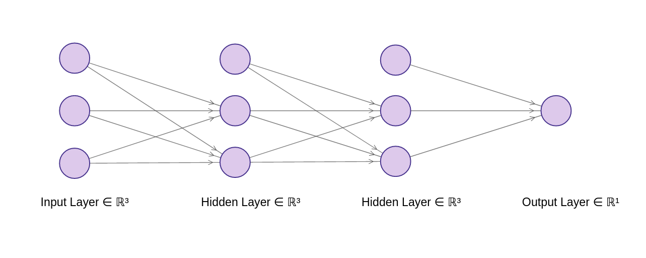
Quick recap of a simple feedforward neural network: Given some training data of form (X, T), where X = input and T = target, we can teach the network what X maps to using the observations / dataset available to us. Remember that the input and target can both be a vector of arbitrarily many dimensions, depending on your data (eg. size of data input to the network below is 2 and output is 1). The goal is to be able to accurately predict what the output will be given some input.
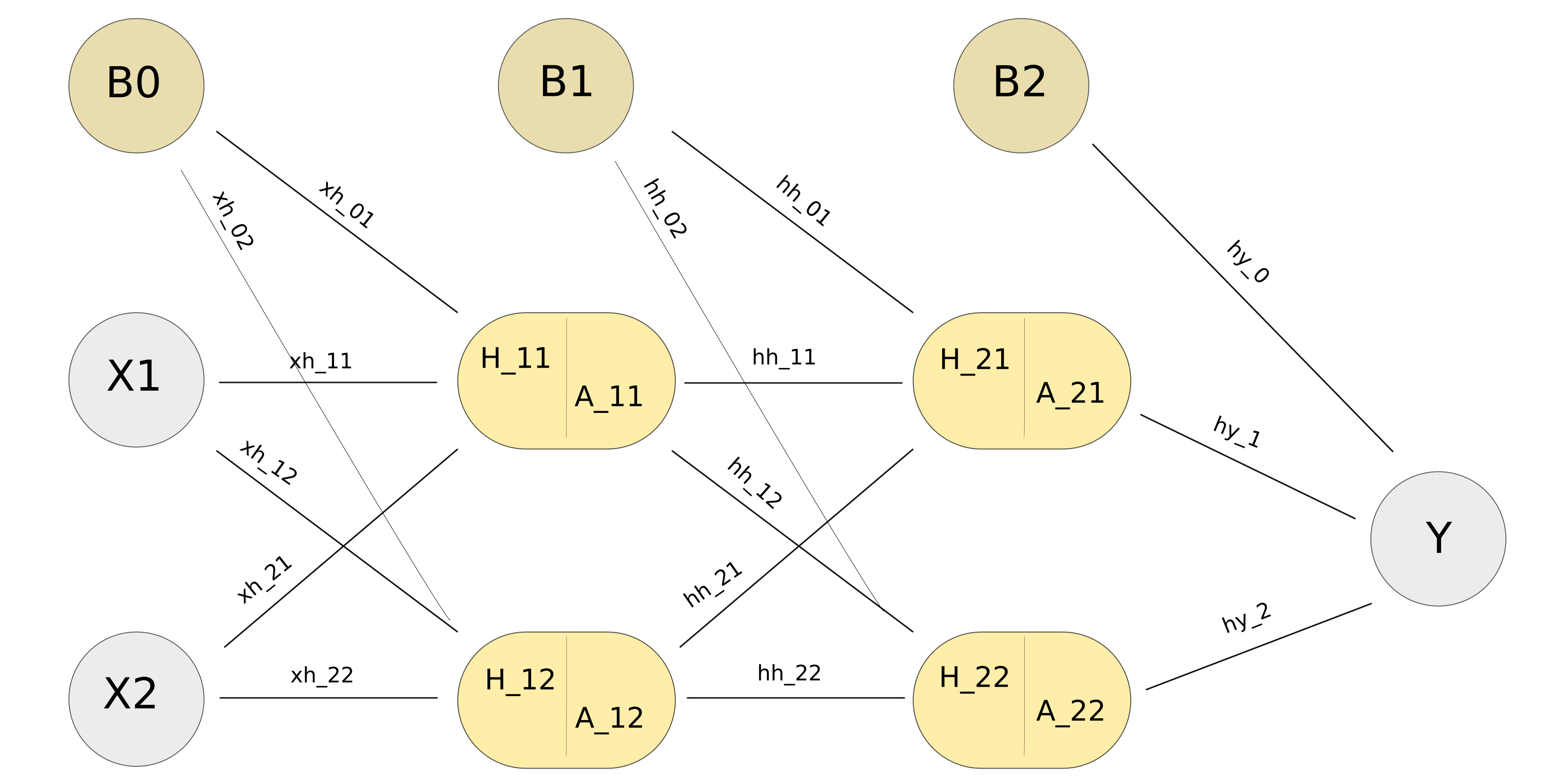
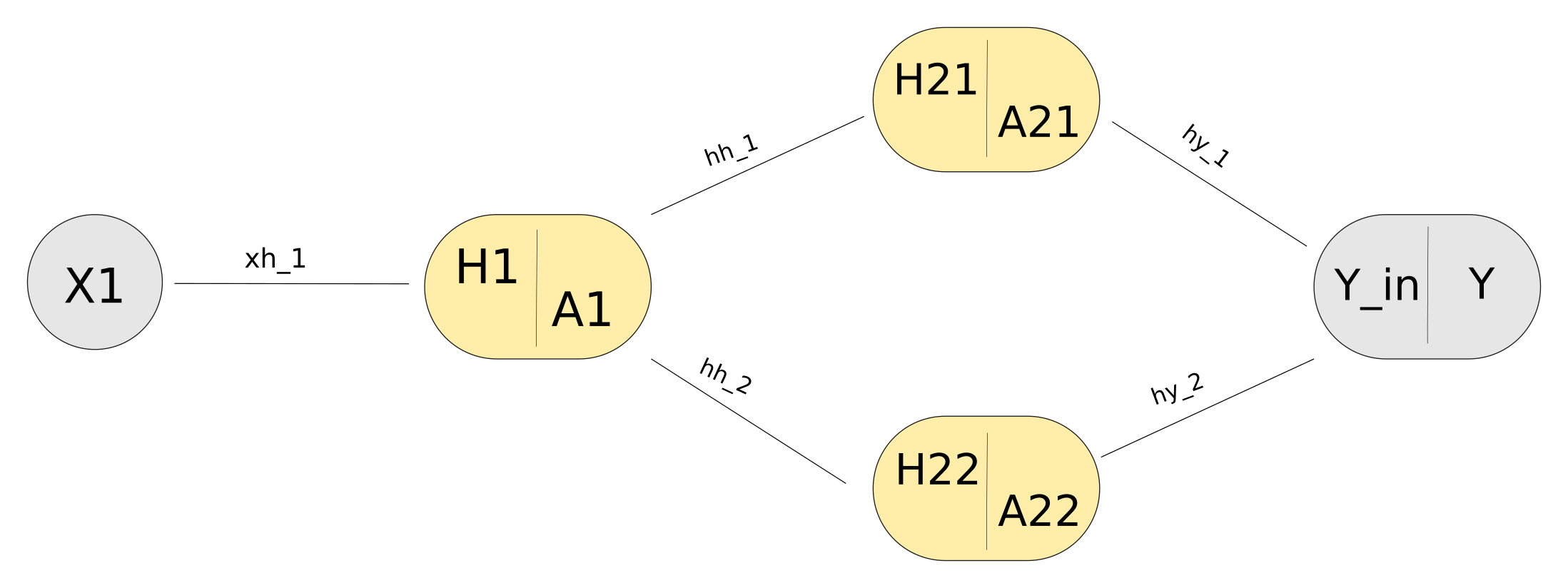
Graphic model of a simple 2 layer feedforward network, with 2 perceptrons in each hidden layer.
- X nodes represents the input
- Weights are smaller labels along edges:
- xh goes from input to hidden layer
- hh goes from hidden to hidden layer
- hy goes from hidden to output layer.
- B nodes are the biases (set to 1, so it is just bias weights that contribute to the next node)
- In the hidden nodes, H denotes the weights multiplied by bias and input from previous layer, summed together (eg. $H_{21} = A_{11}* hh_{11} + A_{12} * hh_{21} + hh_{01}$).
- More formally, $H_j(k) = \sum_i^N O_i(k-1) * w_{ij}$
- i.e. the $j^{th}$ hidden unit of the $k^{th}$ layer is the $i^{th}$ output of the previous layer (output of layer $k-1$, or input X for Layer 1) multiplied by the weight connecting $O_i$ to $H_j$, for all nodes of previous layer and added together.
- A denotes the result after some activation function has been applied to H (eg. $A_{11} = \phi(H_{11})$, where phi represents some activation function).
- Y represents the final output (the thing we are interested in, which should ideally look like T)
The key to the success of the neural network (given that the design is good) lie in the weights. The weights are iteratively changed during training. They minimize some error function that we define, which can be measured by comparing the neural network output (Y) to the desired output (T). There’s some magic that happens in the training step, and then the network can spit out the desired output (hopefully most of the times) when we give it new input data that it has never seen before.
The idea is that we have some number of weights which determine the final output of our network. These weights can be adjusted, and there is some combination of weights which will give us a network output that is closer to the target. When we get closer to the target, we are also getting a lower error, since the difference between the output and target is minimized.
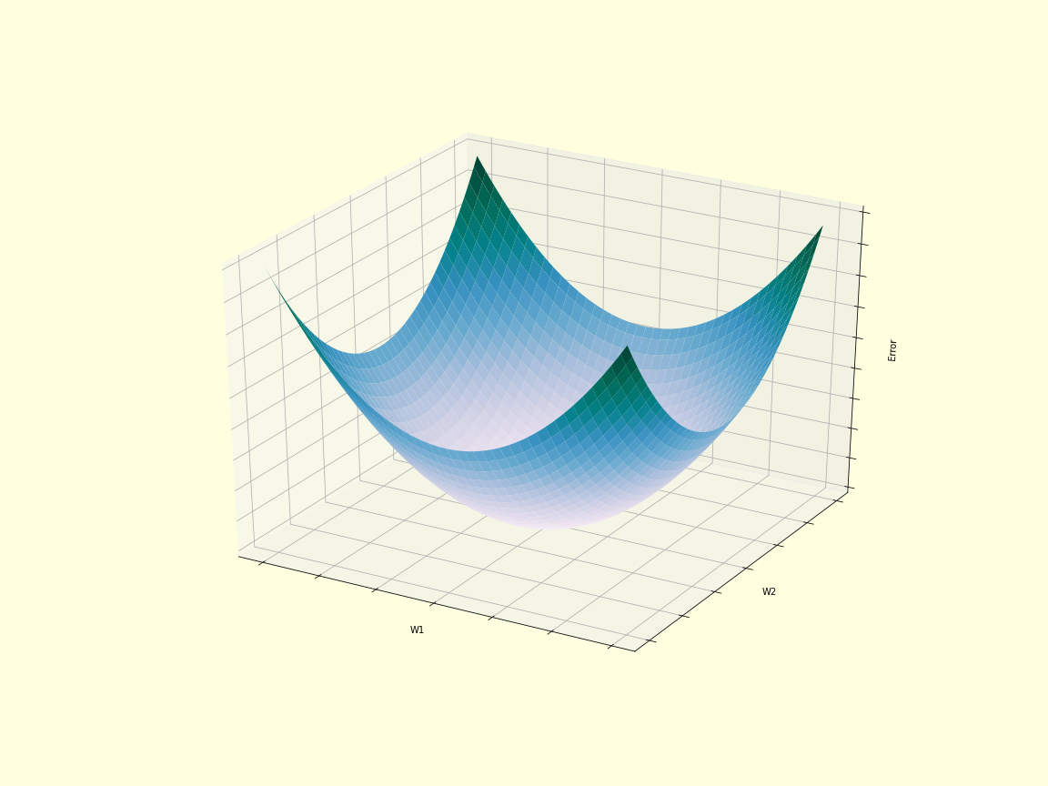
Keep in mind that usually we have more than 2 weights, so it’s usually not feasible to calculate the minimum directly. Instead, we can calculate the gradient of the error function wrt the weights – this gives us the direction to go in order to get to a location of lower error. Remember the derivative gives us the slope of a function. If we have a positive slope, then to go down the slope we have to take a step to the left (going in the negative direction), and vice versa. Since we have many weights, we need partial derivatives wrt each weight. In the 2 weight example, to go down the gradient we take a step along both w1 axis and w2 axis (both weights get changed).
We initialize the weights randomly, so we start off at some random point on the error gradient. Then we calculate which way it slopes at that point and take a step the opposite way to go down the gradient.
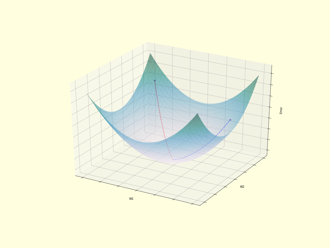
We can get the gradient of the error wrt some particular weight, but we can’t get to it directly when it is an earlier layer since we first compare the target to the output from the last layer in the loss function. If the weight is earlier in the network, we need to go through the layers first and backpropagate the error.
Backpropagation by hand
For purely didactic purposes, we will use a rather unrealistic simple network to demonstrate a weight update (bias weights are left out for simplicity). .
One way to minimize error is to minimize the sum of squares loss function. There are many choices for the loss function, but we’ll choose this one for the examples. This is given by:
$$ L = \frac{1}{2} (Y - T)^2 \tag{1}$$
for the case where Y and T are just single values (otherwise you have to sum over the squared difference between each value in Y and T).
We want to find the gradient of the error function wrt weight $xh_1$. Since this is from an earlier layer, we will make use of the chain rule. I usually think of this as outer function derivative multiplied with derivative of inner function. $\phi$ denotes the activation function, which we will set to $\phi(x) = 2x$ for this example (*this is not normally used as an activation function, afaik, but used here just for simplicity’s sake).
Our output, $$Y = \phi(\,A_{21} * hy_1 + A_{22} * hy_2 \,) \tag{2}$$ can be expanded out even further to include the weight of interest, $xh_1$.
We can rewrite $A_{21}$ out, with green portion representing $A_1$.
$$A_{21} = \phi(hh_1 * \color{green}{\phi(x_1 * xh_1)}) \tag{3}$$
We can do the same thing with $A_{22}$, and plug it all back into Y. Red represents activated hidden units A of layer 2, and blue represents activation for final output Y.
$$ Y = \color{blue}{\phi(}\, hy_1* \color{red}{\phi(} hh_1 * \color{green}{\phi(x_1 * xh_1)} \color{red}{)} + hy_2* \color{red}{\phi(}hh_2 * \color{green}{\phi(x_1 * xh_1)}\color{red}{)}\color{blue}{)} \tag{4}$$
Looking at weight $xh_1$, we can only access it wrt $A_1$, and we have access to $A_1$ wrt nodes in second layer $A_{21}$ and $A_{22}$, and so on.
So using chain rule, we can decompose the loss wrt weight $xh_1$, giving us the error gradient $\nabla L(xh_1)$:
$$ \nabla L(xh_1) =\frac{dL}{dxh_1} = \color{darkblue}{\frac{dL}{dy}} \color{green}{\frac{dy}{dA_2}} \color{orange}{\frac{dA_2}{dA_1}} \color{red}{ \frac{dA_1}{dxh_1}}$$
You may have noticed that there are 2 nodes in layer 2… If you take a look at Y, you’ll see that it is composed of 2 parts, the first portion of the sum goes through node $A_{21}$, and the second through $A_{22}$.
So this can be written as:
$$ \nabla L(xh_1) = \color{darkblue}{\frac{dL}{dy}} \left[ \color{green}{\frac{dy}{dA_{21}}} \color{orange}{\frac{dA_{21}}{dA_1}} \color{red}{\frac{dA_1}{dxh_1}} + \color{green}{\frac{dy}{dA_{22}} } \color{orange}{\frac{dA_{22}}{dA_1}} \color{red}{\frac{dA_1}{dxh_1}} \right] \tag{5}$$
Calculating the individual portions, here we take the derivative of the loss function wrt y:
$$ \frac{dL}{dy} = Y - T = 8 $$
We use $Y_{in}$ to denote the unactivated output (eq. 4 without the activation function).
$$ \frac{dy}{dA_{2i}} = \phi'(Y_{in}) * hy_i \tag{6}$$
The general function for unactivated hidden units & outputs of layer 2:
$$ H_{2i} = hh_i * \color{green}{A_1}$$
$$A_{2i} = \phi(H_{2i}) $$
Taking the derivative wrt $A_1$, the first portion is the derivative of the outer activation function, then the second part is the derivative of the inner part .
$$ \frac{dA_{2i}}{dA_1} = \phi ‘(H_{2i}) * hh_i \tag{7}$$
Finally we can take the derivative of $A_1$ wrt the weight $xh_1$, which just gives us the outer derivative of the activation, and the inner derivative wrt the weight just gives us the input linked to that weight. If you have an input of larger dimension, eg. $X = [x_1, x_2,…x_n]$, then the derivative wrt $w_{ij}$, which links $i^{th}$ input to $j^{th}$ hidden node, would be $x_i$.
$$ \frac{dA_{1}}{dxh_1} = \phi ‘(H_1) * x_1 \tag{8}$$
Putting it all together:
$$ \nabla L(xh_1) = (Y-T) \left[ \color{green}{\phi’(Y_{in}) * hy_1} * \color{orange}{ \phi ‘(H_{21}) * hh_1} * \color{red}{ \phi ‘(H_1) * x_1} \\ + \color{green}{\phi’(Y_{in}) * hy_2} * \color{orange}{ \phi ‘(H_{22}) * hh_2} * \color{red}{ \phi ‘(H_1) * x_1} \right] \tag{9}$$
After we get the error gradient wrt the weight, the change of the weight is the gradient multiplied with a small number which represents the step size or learning rate, denoted by $\eta$.
$$ w_{new} = w_{old} - \eta \, \nabla L(xh_1) \tag{10}$$
Try looking for a pattern in eq. 9. You may also see the change of weight equation in the following format below, which is a nice recursive form that is better for programming (because after learning it, you won’t be doing much backpropagation by hand!).
$$\Delta w_{ij} (k, k+1) = \delta_j(k+1) \; o_i(k) \tag{11}$$
This is a general equation for the weight going from node $i$ in layer $k$ to node $j$ in layer $k+1$, where $ o_i(k) $ is the output from the $i^{th}$ node of the previous layer, and $\delta_j(k+1)$ can be thought of as the error term from the next layer.
For where $k+1$ is a hidden layer:
$$ \delta_i (k) = \phi’(k) \sum_{j=1}^{N(k+1)} w_{ij} (k, k+1) \; \delta_j (k+1) \tag{12}$$
For the final output layer, since it is already the last layer and there is no $k+1$ for the part after the sum, we replace it with the total error (derivative of loss wrt Y).
Using this method, with k=1 representing the first hidden layer and k=3 for the output layer:
$$ \delta(3) = \phi’(Y_{in}) * (Y - T) $$
$$ \delta_1(2) = \phi’(H_{21}) * hy_1 * \delta(3)$$
$$ \delta_2(2) = \phi’(H_{22}) * hy_2 * \delta(3)$$
$$ \delta(1) = \phi'(H_1) * [hh_1 * \delta_1(2) + hh_2 * \delta_2(2)]$$
Plugging this in to eq. 11 for weight $xh_1$, which connects from input layer 0 to hidden layer 1. $o_i(k)$ is just the input.
$$\Delta w_{xh}(0,1) = \delta(1) * x_1 $$
$$ \Delta w_{xh}(0,1) = x_1 * \phi'(Y_{in}) * (Y - T) * (hh_1 * \phi'(H_{21}) * hy_1 \\ + hh_2 * \phi'(H_{22}) * hy_2 ) \tag{13}$$
We simplified eq. 13 by pulling a few terms out, but compare it with eq. 9 and you’ll see it’s the exact same!
We repeat the update for all the weights, then continue iterating between the forward pass, backpropagation of error, and changing the weights, until we’re happy with the result (error is low enough, or not decreasing much more).
Continuing with our example with actual values:
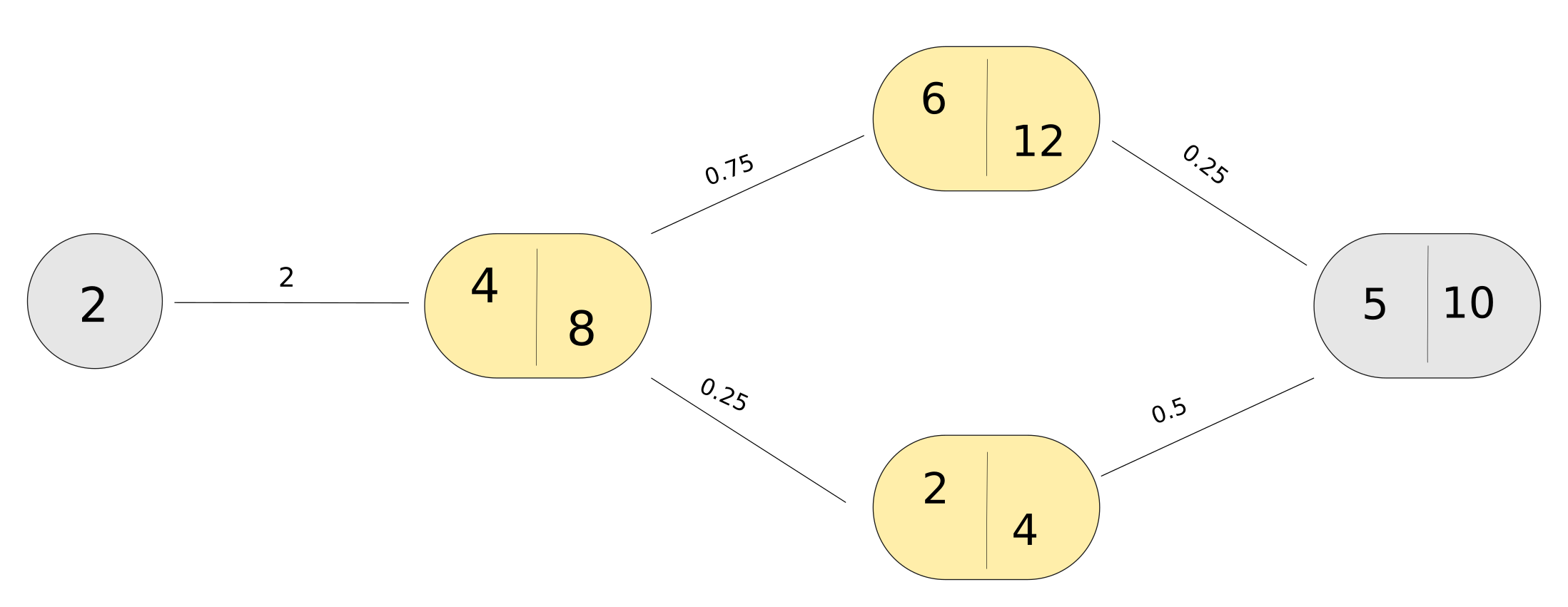
For the input and target of our simple network, X = 2, and T = 2. We calculate the values using eq. 9 and plug it in. Since the activation function $\phi(x) = 2x$, the derivative $\phi'(x) = 2$.
$$ \frac{dy}{dA_{21}} = 2 * 0.25 = 0.5 $$
$$ \frac{dy}{dA_{22}} = 2 * 0.5 = 1 $$
$$\frac{dA_{21}}{dA_1} = 2 * 0.75 = 1.5 $$
$$ \frac{dA_{22}}{dA_1} = 2 * 0.25 = 0.5$$
$$ \frac{dA_{1}}{dxh_1} = 2 * 2 = 4 $$
Plugging everything in:
$$\nabla L(xh_1) = 8 * [0.5 * 1.5 * 4 + 1 * 0.5 * 4] = 40 $$
It looks like the error gradient wrt $xh_1$ is strongly positive, so we should take a step in the opposite direction to go down the gradient. Of course, our learning rate is usually small enough to make sure we don’t make such a drastic leap (because then we might overjump the minimum – imagine crossing over to the other side of the paraboloid and increasing in error again.)
Say we set the learning rate to $\eta$ = 0.03, then the new weight will be
$$ xh_1^{(new)} = xh_1^{(old)} - \eta \, \nabla L(xh_1) $$
$$ = 2 - 0.03 * 40 = 0.8 $$
With a smaller weight, another forward pass would mean a lower output. With just one weight update, we get an output of 4 with a forward pass, which means an error of 2 – much lower than what we had before at 8!
I hope this helped in bettering you understanding of gradient descent and the backpropagation algorithm. Please comment below if you have questions/suggestions or spot any mistakes.
See you next time! 🙂