We’ll explore Gaussian Processes (GPs) through examples written mostly in Python. You can find the jupyter notebook for the images and Octave code here. If you are not familiar with regression or multivariate Gaussians (MVGs), you should brush up on those topics first. This post will go into the intuition and implemention of GPs, and sampling from GP priors using 1D data. Part 2 will cover 2D input data and prediction. Maybe by the end you’ll also appreciate the beauty and cool factor of gaussian processes 😉
Introduction
A common goal in machine learning is to make predictions given data, either through regression or classification (ie. for continuous or discrete predictions). In short, we have some data, and we want some model based on observed data points in order to make predictions for new points. Basically:
$$ data \rightarrow model \rightarrow prediction $$
Gaussian Processes are a class of methods which can be used for prediction and modelling in both regression and classification. We’ll mostly look at how it does it for regression in this and the follow-up post.
Given some data, we assume there’s some underlying function generating this data. We don’t know what this function is, but it would be useful to have some approximation in order to predict for new cases. That’s where regression comes in. We want some approximate function fitted to the data that can best predict for new points.
To find the underlying function using regression, we could take the strategy of restricting the shape of the function by only considering a certain class of functions (eg. linear, polynomial, etc), and try to find the one with the best fit to our data.
Alternatively, we don’t limit ourselves to a particular function type, but instead have a prior over all functions. Now we’re working in the function space, and this is where GPs come in.
Let’s take an example where we only have one observed data point. In this situation, you can imagine that there are many functions that could be generating this point - an infinite amount, actually. Imagine now we have several known data points, which reduces the world of possible functions to only those functions which could pass through all of our observed points. This is where GPs come in. They give us a mechanism for placing a prior over the underlying process and noise as well as for generating new functions.
Function space view
A GP is basically a distribution over functions, where we can think of the input and output space as that of a D-dimensional multivariate Gaussian (MVG). Since we can have an infinite dimensional multivariate Gaussian, this means we can draw an output and plot it as an infinitely long vector, which can essentially be seen as a function.
It is helpful to think of a function as a long vector, where there is an output $y$ for each input $x$. You can imagine that if we have some data, and we think of the observed points as generated by an underlying function plus noise, then the underlying function can be thought of as an infinitely long vector of inputs and outputs.
For intuition of how we draw a function from our prior in function space, say we have a MVG of dimension D, and we draw a point. That point consist of D dimensions. We plot the drawn values $\mathbf{y}$ against the input values $\mathbf{x}$ with each dimension along the x-axis. Since the covariance matrix determines the relation between the values of $\mathbf{x}$, points close to each other on the x-axis are more correlated (closer value in output), so we get a a smooth looking curve. Since we can theoretically draw a point of infinite dimension and plot the output against the input, this can be viewed as a function.


But generally when we have to make predictions, we won’t have to look at the function for all input points… we are only interested in some subset. Since we only need a finite set of points or a certain stretch of the function, this makes it computationally tractable.
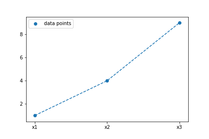
To help with intuition, let’s look at a very simple example. Let’s say we have 3 data points generated by some underlying function (in this case, $f(x) = x^2$). We can also use a MVD to draw and plot points. Imagine drawing a point from a 3D multivariate Gaussian.
Based on the mean and the covariance matrix we set, we have a certain probability of drawing each value at each dimension of the MVG. The formula for the MVG is:
$$ N(x|\mu, \Sigma) = \frac{1}{(2\pi)^{D/2}} \frac{1}{|\Sigma|^{1/2}} exp \Big\{ -\frac{1}{2} (x - \mu)^T \Sigma^{-1} (x - \mu) \Big\}$$
With the input vector, mean vector, and covariance matrix of form:
$$ x = \begin{bmatrix} x_1 \\ x_2 \end{bmatrix} \qquad \mu = \begin{bmatrix} \mu_1 \\ \mu_2 \end{bmatrix} \qquad \Sigma = \begin{bmatrix} \Sigma_{11} & \Sigma_{12} \\ \Sigma_{21} & \Sigma_{22} \end{bmatrix} $$
We can get a conditional distribution of form:
$$ p(x_{1|2}) = N(\mu_{1|2}, \Sigma_{1|2})$$
where
$$ \mu_{1|2} = \mu_1 + \Sigma_{12}\Sigma_{22}^{-1} (x_2 - \mu_2)$$
$$\Sigma_{1|2} = \Sigma_{11} - \Sigma_{12}\Sigma_{22}^{-1}\Sigma_{21}$$
The nice thing about the MVG is that the conditional distribution is another Gaussian. 😌

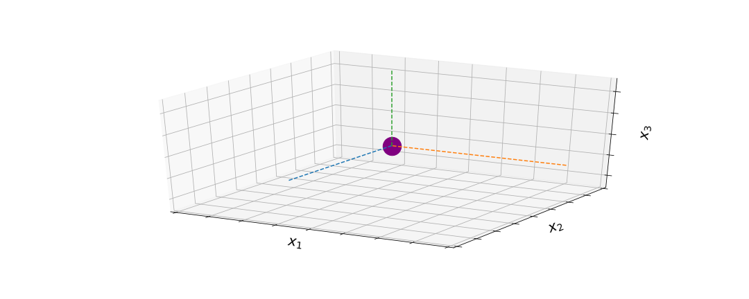
The first image shows what is happening with a sample – there is a certain probability of drawing a value for each dimension. However, this probability changes if we already drew the value for the 2nd dimension – then we are looking at the conditional distribution for drawing the value of the 1st dimension. So imagine we sampled a value for $x_2$ already. Now we have to consider the conditional probability of $x_1$ given $x_2$, $ \: p(x_{1|2}) \,$, which is just another Gaussian distribution.
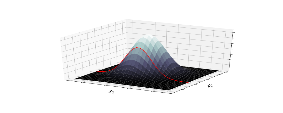
The covariance matrix determines how much the draw of one value affects the next. After drawing a value for $x_2$, we now have a conditional gausssian distribution (red line) that determines the probability of our draw for $x_1$.
Time for some definitions:
A Gaussian process is a generalization of the Gaussian probability distribution. Whereas a probability distribution describes random variables which are scalars or vectors, a stochastic process governs the properties of functions.
A Gaussian process is a collection of random variables, any finite number of which have a joint Gaussian distribution.
We can now break apart the definitions, as we see from previous examples how GPs rely on the Gaussian probability distribution, and is a stochastic process (a collection of random variables indexed by the MVG dimensions). We can also now see how it is a a collection of random variables, in that it can be drawn from a MVG, and the probability of the values of all the variables being drawn together is the joint probability.
Briefly on kernels:
We won’t go into too much detail on kernels in this post, but it is an important part of GPs since it determines our covariance matrix. We can choose a kernel for calculating the covariance matrix of our MVG.
In the examples, we use a widely used kernel given by the exponential of a quadratic form, with constant and linear terms [1]:
$$ k(x_n, x_m) = \theta_0 exp{ -\frac{\theta_1}{2} | x_n - x_m |^2 } + \theta_2 + \theta_3 x_n^Tx_m $$
The covariance matrix (shape $D$ by $D$) calculates the relation between all datapoints using the kernel function, with the variance being along the diagonal, $ \, k(x_i, x_i)$.
Filling the covariance matrix in python code, for an example with 3 datapoints:
|
|
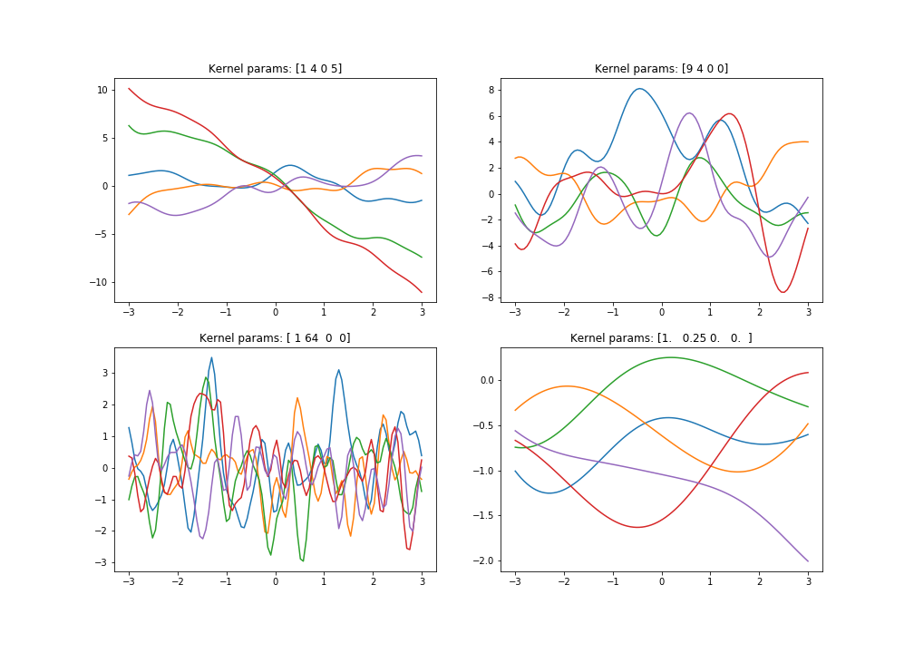
With the kernel parameters we can favour certain types of functions (eg. smoother or more wiggly due to higher/lower covariance) by adjusting the values of **$\theta$**s . If there’s a higher covariance between the input points, they are more dependent, meaning the sample of the next value will be closer to the sample of the previous, thus giving us a smoother function. Take a look below at what happens to sampled functions when we use different kernel parameters.
Drawing functions from the prior with 1D data
Code for sampling 1 function:
|
|
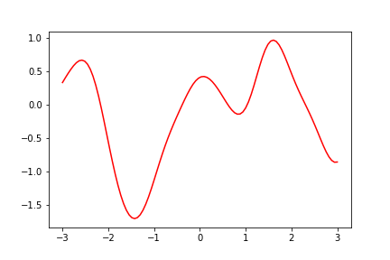
So we drew a random function using our prior with mean vector of zero, but we can also adjust the mean to give us the shape of a particular function. Then our prior samples will look more like our chosen distribution.
How is this function sampled? We use zero mean for all the points. We take the input points we want to use for plotting the function (some evenly spaced vector of points), calculate the covariance matrix using our chosen kernel with our hyperparameters theta which control how strongly correlated the points are with each other. Now using our covariance matrix calculated with our kernel and zero vector as mean, we can sample the output values using our input datapoints. The point we sample will be more likely to be close to the mean value (in this case 0), but it will also depend on the other points sampled (remember the conditional Gaussian above).
If the first point we sample is by chance a bit far from the mean, then for the second point we are more likely to sample closer to the first point as well as the mean of the second point. Just imagine that we are sampling a random variable in high dimensional space, where the dimension is the number of input points.
Part II will cover prior function sampling using 2D input data as well as prediction. The link will be available once published.
Please comment below if you have any questions, feedback, or suggestions for this post 🙂
References
- C. M. Bishop, Pattern Recognition and Machine Learning, Springer, 2006, ISBN-13: 978-0387-31073-2©2006 Springer Science+Business Media, LLC. www.microsoft.com/en-us/research/uploads/prod/2006/01/Bishop-Pattern-Recognition-and-Machine-Learning-2006.pdf
- C. E. Rasmussen & C. K. I. Williams, Gaussian Processes for Machine Learning, the MIT Press, 2006, ISBN 026218253X.c©2006 Massachusetts Institute of Technology. www.GaussianProcess.org/gpml