Variational Inference in Theory

This post will explain what Variational Inference is about (TLDR: it’s a method to approximate the elusive posterior distribution). We’ll get past those tricky hairy math details with some nicer to read color-coded hairy math. Enjoy 😏 ​

Why Variational Inference?

Before we dive into it, first a quick recap of Bayesian Inference. Remember Bayesian Inference is a statistical method which uses Bayes' theorem to update the probability of our hypothesis as we get more data, and can compute the posterior probability of our model parameters.

$$ \color{darkblue}{p(z|D)} =\frac{ \color{green}{p(D|z)} \, \color{orange}{p(z)}} { \color{brown} {p(D)}}$$

This formula is saying that our posterior equals the likelihood times the prior over the marginal or evidence.

From a graphical model perspective, we can imagine that some underlying latent variable $z$ is influencing our observed variables $D$.

We have the data, and we’re trying to model the underlying data generating process. For the formulation of our problem, the posterior is like asking the question, what is the probability of $z$ given our data $D$? It could also represent the unknown parameters for the model we’re trying to fit to our data.

In order to get the marginal distribution $\color{brown} {p(D)}$, we need to integrate over all possible $z$s, and in doing so we marginalize out the $z$ and end up with just $\color{brown} {p(D)}$.

$$ \color{brown}{\color{brown} {p(D)}} = \int \color{teal}{p(D,z)} dz = \int \color{green}{p(D | z)} \color{orange}{p(z)} dz $$

This integral is often not possible to compute. Perhaps it is feasible if $p(D|z)$ and $p(z)$ are conjugate distributions or you have a very simple model, but often times it is ugly and difficult, if not downright impossible to compute.

This is where Variational Inference (VI) comes to save the day ☀️. It tries to approximate the conditional posterior distribution, skipping over the integration hassles by turning this into an optimization problem.

Granted, there are other ways for us to tackle the intractable marginal distribution of the posterior, the difficult normalizing denominator which is our missing piece to a true posterior probability distribution. We can use MCMC methods such as Gibbs Sampling or Metropolis Hastings, which can approximate the posterior distribution by sampling from the unnormalized posterior. These methods can be easier to understand and a bit more straightforward. However, sampling methods can take a long time to converge. VI is good for getting a quicker approximation, sacrificing preciseness for efficiency.

How it works:

So the problem is that we can’t solve the integral in the denominator, thus we don’t have our posterior distribution $\color{darkblue}{p(z|D)}$. The solution proposed by VI is to approximate $\color{darkblue}{p(z|D) }$ with another distribution, $\color{darkorchid} {q(z)}$, and thus bypassing the intractable integral.

Let’s say we have some parameters, which we can tweak to make our new distribution $\color{darkorchid} {q(z)}$ as close to $p(z|D)$ as possible. Where do we start? We want to convert this into an optimization problem, where we can use optimization methods to get the approximate distribution close to the true distribution. To do that, we need to have a measure to know when we are getting closer to the true posterior.

Kullback–Leibler (KL) Divergence

Thankfully, we can measure the similarity of two distributions using the KL Divergence. You can calculate it with:

$$ KL(Q \Vert P) = \sum_{z \in Z} \color{darkorchid} {q(z)} \, log \Big( \frac{\color{darkorchid} {q(z)}}{ \color{darkblue}{p(z|D)} } \Big)\tag{1} $$

In the case of continous distributions, use an integral instead:

$$ KL(Q \Vert P) = \int_{-\infty}^\infty \color{darkorchid} {q(z)} \, log \Big( \frac{\color{darkorchid} {q(z)}}{ \color{darkblue}{p(z|D)} } \Big) dz \tag{2}$$

Applying the log rule, you can reformulate eq. 2 as:

$$ KL(Q \Vert P) = - \int_{-\infty}^\infty \color{darkorchid} {q(z)} \, log \Big( \frac{ \color{darkblue}{p(z|D)} }{\color{darkorchid} {q(z)}} \Big) $$

Which can be equivalently seen as:

$$KL(Q \Vert P) = \int_{-\infty}^\infty \color{darkorchid} {q(z)} \; log(\color{darkorchid} {q(z)}) - \int_{-\infty}^\infty \color{darkorchid} {q(z)} \; log( \color{darkblue}{p(z|D)} ) \tag{3}$$

A few things to keep in mind:

KL divergence is non-negative: $ KL(Q \Vert P) \ge 0 $, see Information Theory box below for explanation.

KL distance is not symmetric: $KL(Q \Vert P) \neq KL(P \Vert Q)$, with the first being reverse KL and the latter called forward KL.

Look at the KL formula in eq. 2 once more and get a feeling for it. Intuitively:

• If $\color{darkblue}{p(z|D)}$ and $\color{darkorchid} {q(z)}$ are similar, the log term would be low so KL is low – good 😄
• if $\color{darkorchid} {q(z)}$ is high and $\color{darkblue}{p(z|D)}$ is low, then KL is high – bad 😞
• if $\color{darkorchid} {q(z)}$ is low and $\color{darkblue}{p(z|D)}$ is high, then KL is still low as it is weighted with $\color{darkorchid} {q(z)}$

Visualizing the difference between forward and reverse KL:¹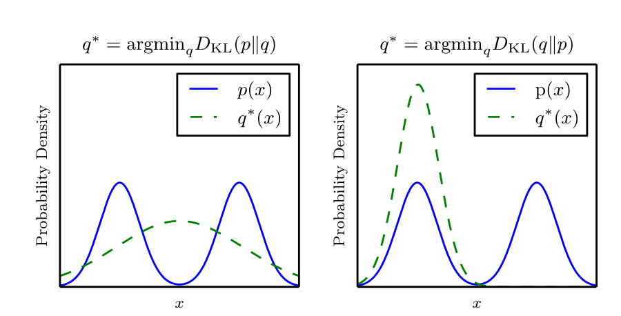

When we use reverse KL, $\color{darkorchid} {q(z)}$ is forced to be low for whenever $\color{darkblue}{p(z|D)}$ is low since we want the lowest possible KL divergence, meaning in areas of low probability for $\color{darkblue}{p(z|D)}$, then $\color{darkorchid} {q(z)}$ would also be low. This leads to mode-seeking behaviour where it might only capture one mode in a multi-modal distribution. With forward KL, it doesn’t matter if $\color{darkorchid} {q(z)}$ is high where $\color{darkblue}{p(z|D)}$ is low, since the KL is still low when weighted with $\color{darkblue}{p(z|D)}$.

So what does entropy and cross entropy have to do with KL divergence? Well, the lowest possible cross-entropy would be equal to the self entropy, when the 2 distributions are the same: $p(x) = q(x)$. KL divergence measures how similar the 2 distributions are, so we can just look at the difference between the cross-entropy and the entropy. When the distributions are the same, then the difference should be 0. We want our approximate distribution $q(x)$ to be as close to $p(x)$ as possible, and we can measure the distance by taking the difference between the cross entropy of the approximate and true distributions and the entropy of the true distribution. The larger the difference, the more dissimilar are the two distributions.

$$ KL(p \Vert q) = H(p, q) - H(p) $$

Take a look again at equation 3. See the connection?

The cross entropy must be higher or equal to the entropy, $ H(p,q) \ge H(p)$, if equal then the distributions are the same which gives us a distance of zero (check out Gibbs' Inequality).

This is why KL divergence is always non-negative, and it is only zero when the two distributions are the same: $ KL(p \Vert q) = 0 \iff p(x) = q(x)$.

We almost have the equation to do optimization with. It would be great if we could just minimize the KL divergence between the two distributions directly, but we can’t quite yet because we don’t actually have $ \color{darkblue}{p(z|D)} $ to calculate the KL divergence with. We can tweak the KL divergence a bit and use the joint probability instead.

In short, working with KL directly is cumbersome, so we do some math and find a better term for optimization.

The ELBO

An equivalent to minimizing the KL divergence is to maximize the evidence lower bound (ELBO). Let’s take a look again the eq. 2 for KL divergence:

$$ KL(Q \Vert P) = \int_{-\infty}^\infty \color{darkorchid} {q(z)} \, log \Big( \frac{\color{darkorchid} {q(z)}}{ \color{darkblue}{p(z|D)} } \Big) dz $$

To get rid of the conditional posterior $p(z | D)$, we can substitute it with something equivalent. We can use the property:

$$ \color{darkblue}{ \color{darkblue}{p(z|D)} } = \frac{\color{teal}{\color{teal}{p(z,D)}}}{\color{brown} {p(D)}} $$

Substituting in, we get:

$$ KL(Q \Vert P) = \int_{-\infty}^\infty \color{darkorchid} {q(z)} \, log \Big( \frac{\color{darkorchid} {q(z)} \, \color{brown} {\color{brown} {p(D)}}}{\color{teal}{p(z,D)}} \Big) dz \tag{4}$$

We can pull out $\color{brown} {p(D)}$, getting:

$$ KL(Q \Vert P) = \int_{-\infty}^\infty \color{darkorchid} {q(z)} \, log \Big( \frac{\color{darkorchid} {q(z)}}{\color{teal}{p(z,D)}} \Big) dz + \underbrace{ \int_{-\infty}^\infty \color{darkorchid} {q(z)} }_{\text{integrates out}} \, log(\color{brown} {p(D)}) dz \tag{5}$$

In the right-hand portion, since $log( \color{brown} {p(D)})$ is not dependent on $z$, we can remove the integral since $ \int_{-\infty}^\infty \color{darkorchid} {q(z)} \, dz = 1$ . This leaves us with:

$$ KL(Q \Vert P) = \underbrace{ \int_{-\infty}^\infty \color{darkorchid} {q(z)} \, log \Big( \frac{\color{darkorchid} {q(z)}}{\color{teal}{p(z,D)}} \Big) dz }_{\text{neg. ELBO}} + log(\color{brown} {p(D)}) \tag{6}$$

This leads us to an equation that only depends on the joint $\color{teal}{\color{teal}{p(z,D)}}$, and not $p(z|D)$ . The term on the right hand side is actually the negative ELBO. With this reformulating, we see that the KL divergence is the equivalent to the negative ELBO up to some constant, $log(\color{brown} {p(D)}$, as it does not depend on $z$. This means that if we want to minimize the KL, we’re doing the opposite to the ELBO. Let’s rearrange the equation a bit to see this better.

$$ log(\color{brown} {p(D)}) = KL(Q \Vert P) \, \underbrace{ - \, \int_{-\infty}^\infty \color{darkorchid} {q(z)} \, log \Big( \frac{\color{darkorchid} {q(z)}}{\color{teal}{p(z,D)}} \Big) dz }_{\text{ELBO}} \tag{7}$$

$$ = KL(Q \Vert P) + ELBO $$

Remember that optimization depends on going towards the location where the change with respect to $z$ is 0, as that will be either a maximum or minimum point. Both KL and ELBO depend on $z$, but we can just look at $log(\color{brown} {p(D)})$ as some constant since it has no dependency on $z$. As $log(\color{brown} {p(D)})$ is just a constant, we can see that the two components balance each other $\Rightarrow$ KL is smaller when ELBO is larger, and vice versa.

However, since KL is non-negative, this means that ELBO must be smaller than or equal to the marginal likelihood $log(\color{brown} {p(D)})$, also known as model evidence. And that’s why we call it the Evidence Lower Bound, since it’s a lower bound on the marginal log likelihood of the data.

Mean field approximation

To use VI, we want to find a tractable distribution family to use so we can actually calculate $\color{darkorchid} {q(z)}$ and $\color{teal}{p(z,D)}$.

We can make an assumption to make $\color{darkorchid} {q(z)}$ tractable when we have many latent variables, by assuming independence of the latent variables $z$ so that it can factorize:

$$ q(z_1 … z_m) = \prod_{i=1}^{M} q(z_i) \tag{8}$$

One way to optimize the ELBO is by using coordinate ascent (optimize ea. latent variable’s approximation $q(z_i)$ in turn while holding others fixed). There are also other ways like typical gradient optimization methods.

Note that expectation can be defined as:

$$E_{g}[f(x)] = \int g(x) \, f(x) \,dx$$

Using log rules and expectation, our ELBO from eq. 7 can also be written as:

$$ L = \color{darkblue}{E_q[log \, p(z,D)]} - \color{brown}{E_q[log(q(z))]} \tag{9}$$

Using the assumption we made in eq. 8, we can write the second term as:

$$ \color{brown}{E_q[log(q_{i:m})]} = \sum_i^m E_{q_i}[log(q(z_i))] \tag{10}$$

Let’s take a look now what we can do with the first piece. Using the chain rule, we decompose the joint into:

$$ \color{darkblue} {p(z,D)} = \color{purple}{p(z|D)} \color{green}{p(D)}$$

Our data is composed of $D = x_{1:N}$ and we have $z_{1:M}$ latent variables, which gives us:

$$\color{darkblue}{p(z_{1:M}, x_{1:N})} = \color{green}{p(x_{1:N})} \color{purple}{ \prod_i^M p(z_i | z_{1:(i-1)}, x_{1:N})} \tag{11}$$

$$ \color{darkblue}{log \, p(z_{1:M}, x_{1:N})} = \color{green}{log \, p(x_{1:N})} + \color{purple}{\sum_i^M log \,p(z_i | z_{1:(i-1)}, x_{1:N})} $$

Described in plain words, we have the log probability of all the data $p(x_{1:N})$ multiplied with the conditional probabilities of each latent variable $z_i$ given all the data $x_{1:N}$, and all the other latent variables $z_{1:(i-1)}$. The notation $z_{1:(i-1)}$ represents all the other variables because after selecting $z_i$, we move it to the very end so it is the last variable in the list.² Alternatively, we can use the notation $z_{1:(i-1)} = z_{\neg i}$ to represent all the latent variables excluding the $i^{th}$ one.

Now we can put the terms together back into the ELBO:

$$ L = \color{darkblue}{log \, p(x_{1:N}) + \sum_i^M E_q[log \,p(z_i | z_{\neg i}, x_{1:N})]} - \color{brown}{\sum_i^M E_{q_i}[log \, q(z_i)]} \tag{12}$$

In case you’re wondering where the expectation went for $log(p(x))$: since it does not depend on $z$, the expectation using $\color{darkorchid} {q(z)}$ integrated to 1 and it was left by itself. Since it does not depend on $z$, it is viewed as just a constant $K$. This gives us the objective function to do optimization with:

$$ L_i = \color{darkblue}{E_q[log \,p(z_i | z_{\neg i}, x_{1:N})]} - \color{brown}{E_{q_i}[log \, q(z_i)]} + K \tag{13}$$

To maximize $L$, we look at where the derivative of the function goes to 0. Let’s rewrite the equation so we can take the derivative with respect to $q(z_i)$. Remember that $z_{\neg i}$ stands for all indices of $z$ except the $i^{th}$.

Pulling out the term with $q(z_i)$:

$$ L_i = \color{darkblue}{\int \prod_i^M q(z_i) \, log \, p(z_i | z_{\neg i}, x_{1:N} ) dz_{i…m}} - \color{brown}{\int q(z_i) \, log \, q(z_i) \, dz_i}$$

$$ L_i = \color{darkblue}{\int q(z_i) \, \int \prod_{\neg i}^M q(z_{\neg i}) log \, p(z_i | z_{\neg i}, x_{1:N} ) dz_{\neg i} dz_i} - \color{brown}{\int q(z_i) \, log \, q(z_i) \, dz_i}$$

$$ = \color{darkblue}{\int q(z_i) \, E_{\neg i}[log \, p(z_i | z_{\neg i}, x_{1:N} )] dz_i} - \color{brown}{\int q(z_i) \, log \, q(z_i) \, dz_i} \tag{14}$$

Taking the derivative and setting it to zero:

$$ \frac{dL_i}{d q(z_i)} = \color{darkblue}{E_{\neg i}[log \, p(z_i | z_{\neg i}, x_{1:N} )]} \color{brown}{-log\,q(z_i) - 1} = 0 \tag{15}$$

Solving for $q(z_i)$:

$$ q^*(z_i) \propto exp(E_{\neg i}[log \, p(z_i|z_{\neg i}, x)]) \tag{16}$$

This is just an approximation because we also had to add in a Lagrange multiplier to ensure that the individual $q(z_i)$ are probability density functions, so there is also a normalization constant we’re ignoring here (for more details on this see the first link below under resources).

The form of $q^*(z_i)$ can be used directly for coordinate ascent. We choose some tractable family of distribution to use, and after plugging in, the normalization constant can also usually be derived. We can:

• start by randomly initiating all the latent $z_i$ parameters for $\color{darkorchid} {q(z)}$,
• then use eq. 16 to update $q^*(z_i)$ one by one until convergence.

We may only converge to a local maximum, but it’s much more computationally efficient than sampling methods for approximating the posterior. So we’re sacrificing some precision for speed.

That’s the general idea, but we can also decompose the ELBO in another way and use gradient methods to update (for example with the deep learning Variational Auto-encoder model, which may be covered in a future post). See you next time!

---

Resources

For a detailed derivation using mean field approximation:

https://bjlkeng.github.io/posts/variational-bayes-and-the-mean-field-approximation/

Next two are lecture notes which are quite similar and both very helpful:

https://www.cs.princeton.edu/courses/archive/fall11/cos597C/lectures/variational-inference-i.pdf

https://www.cs.cmu.edu/~epxing/Class/10708-15/notes/10708_scribe_lecture13.pdf

---

1. graphic from NIPS 2016 Tutorial: Generative Adversarial Networks ↩︎

2. 10-708: Probabilistic Graphical Models 10-708, Spring 2017. Lecture 13 : Variational Inference: Mean Field Approximation ↩︎